Linear Regression, Classification, Clustering

1 Project Overview

1.1 Purpose of Document

The purpose of this document is to provide a comparison between different AI models for a given dataset to determine which models are most accurate. This document also explores what measures can be taken to improve accuracy in various AI models.

1.2 Scope

The scope of the project involves an exploratory examination of a dataset to determine how best to sample and clean the data for AI training and testing purposes. Various data visualizations are needed to properly understand the dataset and how best to proceed with training models. Training of various models and algorithms are required to produce sufficient comparisons with the ultimate goal of improving accuracy.

2 Dataset Exploratory Analysis

2.1 Descriptive Analysis

The dataset used in this project consists of available independent variables for a variety of cars to ascertain how they affect the price. The chosen dataset contains 26 columns and 205 rows of data with no null values. It is a sufficient dataset in terms of size and types of data for use in training univariate & multivariate linear regression, classification and clustering models.

The Columns

• Car_ID : Unique id of each observation (Integer)
• Symboling : Its assigned insurance risk rating, A value of +3 - Indicates that the auto is risky, -3 that it is probably pretty safe.
• carCompany : Name of car company (Categorical)
• fueltype : Car fuel type i.e gas or diesel (Categorical)
• aspiration : Aspiration used in a car (Categorical)
• doornumber : Number of doors in a car (Categorical)
• carbody : Body of car (Categorical)
• drivewheel : Type of drive wheel (Categorical)
• enginelocation : Location of car engine (Categorical)
• wheelbase : Wheelbase of car (Numeric)
• carlength : Length of car (Numeric)
• carwidth : Width of car (Numeric)
• carheight : Height of car (Numeric)
• curbweight : The weight of a car without occupants or baggage. (Numeric)
• enginetype : Type of engine. (Categorical)
• cylindernumber : Cylinder placed in the car (Numeric)
• enginesize : Size of car (Numeric)
• fuelsystem : Fuel system of car (Categorical)
• boreratio : Boreratio of car (Numeric)
• stroke : Stroke or volume inside the engine (Numeric)
• compressionratio : Compression ratio of car (Numeric)
• horsepower : Horsepower (Numeric)
• peakrpm : Car peak rpm (Numeric)
• citympg : Mileage in city (Numeric)
• highwaympg : Mileage on highway (Numeric)
• price(Dependent variable) : Price of car (Numeric)

Code

# Import libraries for analysis and plotting
import pandas as pd
import numpy as np
import matplotlib.pyplot as plt
%matplotlib inline
import seaborn as sns


# Save data in Pandas dataframe
dataset = pd.read_csv("CarPrice_Assignment.csv")

# Print how many rows and columns are in dataset
print('Dataset Shape:',dataset.shape)

# Turn of max columns so that head() displays all columns in dataset
pd.set_option('display.max_columns', None)

pd.set_option('display.max_rows', 5)

# Display 1st five entries of dataset
dataset.head()

Dataset Shape: (205, 26)

	car_ID	symboling	CarName	fueltype	aspiration	doornumber	carbody	drivewheel	enginelocation	wheelbase	carlength	carwidth	carheight	curbweight	enginetype	cylindernumber	enginesize	fuelsystem	boreratio	stroke	compressionratio	horsepower	peakrpm	citympg	highwaympg	price
0	1	3	alfa-romero giulia	gas	std	two	convertible	rwd	front	88.6	168.8	64.1	48.8	2548	dohc	four	130	mpfi	3.47	2.68	9.0	111	5000	21	27	13495.0
1	2	3	alfa-romero stelvio	gas	std	two	convertible	rwd	front	88.6	168.8	64.1	48.8	2548	dohc	four	130	mpfi	3.47	2.68	9.0	111	5000	21	27	16500.0
2	3	1	alfa-romero Quadrifoglio	gas	std	two	hatchback	rwd	front	94.5	171.2	65.5	52.4	2823	ohcv	six	152	mpfi	2.68	3.47	9.0	154	5000	19	26	16500.0
3	4	2	audi 100 ls	gas	std	four	sedan	fwd	front	99.8	176.6	66.2	54.3	2337	ohc	four	109	mpfi	3.19	3.40	10.0	102	5500	24	30	13950.0
4	5	2	audi 100ls	gas	std	four	sedan	4wd	front	99.4	176.6	66.4	54.3	2824	ohc	five	136	mpfi	3.19	3.40	8.0	115	5500	18	22	17450.0

Code

# Print data types and how many null values are present
dataset.info()

<class 'pandas.core.frame.DataFrame'>
RangeIndex: 205 entries, 0 to 204
Data columns (total 26 columns):
 #   Column            Non-Null Count  Dtype  
---  ------            --------------  -----  
 0   car_ID            205 non-null    int64  
 1   symboling         205 non-null    int64  
 2   CarName           205 non-null    object 
 3   fueltype          205 non-null    object 
 4   aspiration        205 non-null    object 
 5   doornumber        205 non-null    object 
 6   carbody           205 non-null    object 
 7   drivewheel        205 non-null    object 
 8   enginelocation    205 non-null    object 
 9   wheelbase         205 non-null    float64
 10  carlength         205 non-null    float64
 11  carwidth          205 non-null    float64
 12  carheight         205 non-null    float64
 13  curbweight        205 non-null    int64  
 14  enginetype        205 non-null    object 
 15  cylindernumber    205 non-null    object 
 16  enginesize        205 non-null    int64  
 17  fuelsystem        205 non-null    object 
 18  boreratio         205 non-null    float64
 19  stroke            205 non-null    float64
 20  compressionratio  205 non-null    float64
 21  horsepower        205 non-null    int64  
 22  peakrpm           205 non-null    int64  
 23  citympg           205 non-null    int64  
 24  highwaympg        205 non-null    int64  
 25  price             205 non-null    float64
dtypes: float64(8), int64(8), object(10)
memory usage: 41.8+ KB

Code

# Display some descriptive statistics
dataset.describe().round(2)

	car_ID	symboling	wheelbase	carlength	carwidth	carheight	curbweight	enginesize	boreratio	stroke	compressionratio	horsepower	peakrpm	citympg	highwaympg	price
count	205.00	205.00	205.00	205.00	205.00	205.00	205.00	205.00	205.00	205.00	205.00	205.00	205.00	205.00	205.00	205.00
mean	103.00	0.83	98.76	174.05	65.91	53.72	2555.57	126.91	3.33	3.26	10.14	104.12	5125.12	25.22	30.75	13276.71
std	59.32	1.25	6.02	12.34	2.15	2.44	520.68	41.64	0.27	0.31	3.97	39.54	476.99	6.54	6.89	7988.85
min	1.00	-2.00	86.60	141.10	60.30	47.80	1488.00	61.00	2.54	2.07	7.00	48.00	4150.00	13.00	16.00	5118.00
25%	52.00	0.00	94.50	166.30	64.10	52.00	2145.00	97.00	3.15	3.11	8.60	70.00	4800.00	19.00	25.00	7788.00
50%	103.00	1.00	97.00	173.20	65.50	54.10	2414.00	120.00	3.31	3.29	9.00	95.00	5200.00	24.00	30.00	10295.00
75%	154.00	2.00	102.40	183.10	66.90	55.50	2935.00	141.00	3.58	3.41	9.40	116.00	5500.00	30.00	34.00	16503.00
max	205.00	3.00	120.90	208.10	72.30	59.80	4066.00	326.00	3.94	4.17	23.00	288.00	6600.00	49.00	54.00	45400.00

2.2 Cleaning

Multiple columns are object data types but for classification and clustering purposes they were converted to category types. Column 16, “cylindernumber”, values were changed from strings to integers to assist in training some of the linear regression models.

Code

# Convert object data types to category types
dataset['CarName'] = dataset['CarName'].astype('category')
dataset['fueltype'] = dataset['fueltype'].astype('category')
dataset['aspiration'] = dataset['aspiration'].astype('category')
dataset['doornumber'] = dataset['doornumber'].astype('category')
dataset['carbody'] = dataset['carbody'].astype('category')
dataset['drivewheel'] = dataset['drivewheel'].astype('category')
dataset['enginelocation'] = dataset['enginelocation'].astype('category')
dataset['enginetype'] = dataset['enginetype'].astype('category')
dataset['fuelsystem'] = dataset['fuelsystem'].astype('category')
dataset['curbweight'] = dataset['curbweight'].astype('int')

# Convert strings to integers in cylindernumber column to potentially use in the regression models
dataset['cylindernumber'] = dataset['cylindernumber'].replace(['two'], 2).replace(['three'], 3)\
.replace(['four'], 4).replace(['five'], 5).replace(['six'], 6).replace(['eight'], 8).replace(['twelve'], 12)

dataset.head()

	car_ID	symboling	CarName	fueltype	aspiration	doornumber	carbody	drivewheel	enginelocation	wheelbase	carlength	carwidth	carheight	curbweight	enginetype	cylindernumber	enginesize	fuelsystem	boreratio	stroke	compressionratio	horsepower	peakrpm	citympg	highwaympg	price
0	1	3	alfa-romero giulia	gas	std	two	convertible	rwd	front	88.6	168.8	64.1	48.8	2548	dohc	4	130	mpfi	3.47	2.68	9.0	111	5000	21	27	13495.0
1	2	3	alfa-romero stelvio	gas	std	two	convertible	rwd	front	88.6	168.8	64.1	48.8	2548	dohc	4	130	mpfi	3.47	2.68	9.0	111	5000	21	27	16500.0
2	3	1	alfa-romero Quadrifoglio	gas	std	two	hatchback	rwd	front	94.5	171.2	65.5	52.4	2823	ohcv	6	152	mpfi	2.68	3.47	9.0	154	5000	19	26	16500.0
3	4	2	audi 100 ls	gas	std	four	sedan	fwd	front	99.8	176.6	66.2	54.3	2337	ohc	4	109	mpfi	3.19	3.40	10.0	102	5500	24	30	13950.0
4	5	2	audi 100ls	gas	std	four	sedan	4wd	front	99.4	176.6	66.4	54.3	2824	ohc	5	136	mpfi	3.19	3.40	8.0	115	5500	18	22	17450.0

Code

# Print new data types and how many null values are present
dataset.info()

<class 'pandas.core.frame.DataFrame'>
RangeIndex: 205 entries, 0 to 204
Data columns (total 26 columns):
 #   Column            Non-Null Count  Dtype   
---  ------            --------------  -----   
 0   car_ID            205 non-null    int64   
 1   symboling         205 non-null    int64   
 2   CarName           205 non-null    category
 3   fueltype          205 non-null    category
 4   aspiration        205 non-null    category
 5   doornumber        205 non-null    category
 6   carbody           205 non-null    category
 7   drivewheel        205 non-null    category
 8   enginelocation    205 non-null    category
 9   wheelbase         205 non-null    float64 
 10  carlength         205 non-null    float64 
 11  carwidth          205 non-null    float64 
 12  carheight         205 non-null    float64 
 13  curbweight        205 non-null    int64   
 14  enginetype        205 non-null    category
 15  cylindernumber    205 non-null    int64   
 16  enginesize        205 non-null    int64   
 17  fuelsystem        205 non-null    category
 18  boreratio         205 non-null    float64 
 19  stroke            205 non-null    float64 
 20  compressionratio  205 non-null    float64 
 21  horsepower        205 non-null    int64   
 22  peakrpm           205 non-null    int64   
 23  citympg           205 non-null    int64   
 24  highwaympg        205 non-null    int64   
 25  price             205 non-null    float64 
dtypes: category(9), float64(8), int64(9)
memory usage: 36.1 KB

2.3 Visualizations

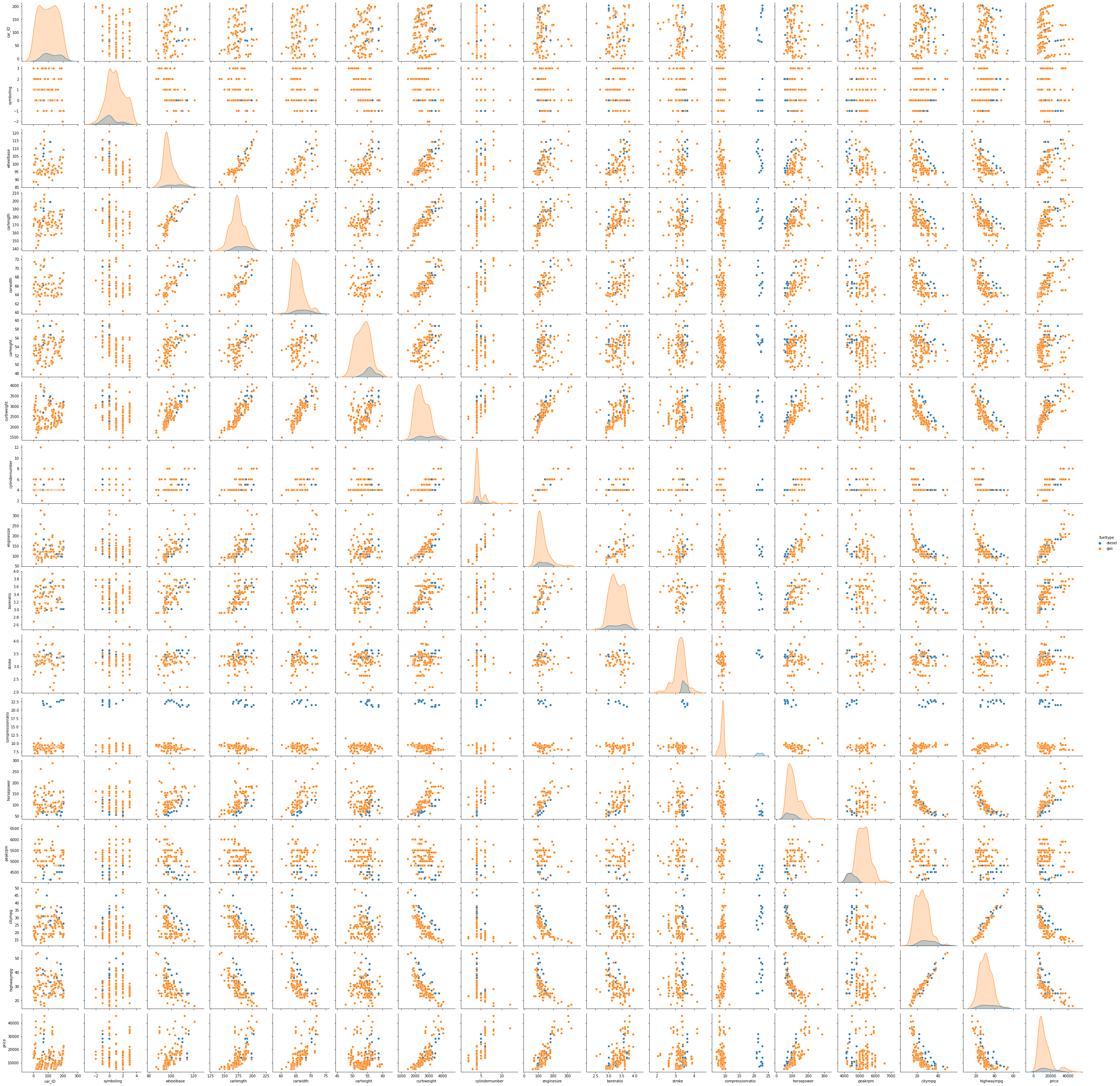
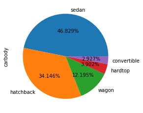
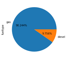
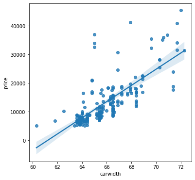
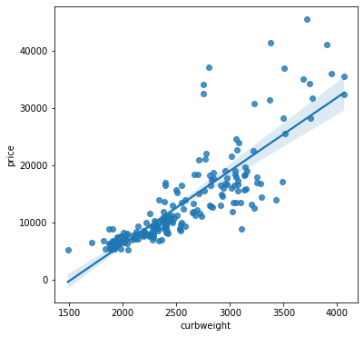
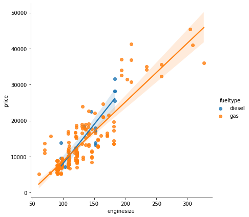
A pairplot ( See Figure 1 ) provides a quick overview of how the variables relate, showing some possibilities for training models. The ‘carbody’ ( See Figure 2 ) and ‘fueltype’ ( See Figure 3 ) columns show promise for use with the classification and clustering models ( See Figure 4 (f) & Figure 4 (g) ). Clear linear relationships exist between ‘carlength’, ‘carwidth’, ‘curbweight’, ‘enginesize’, ‘cylindernumber’ and ‘horsepower’ independent variables and the dependent variable ‘price’ ( See Figure 4 (a) - (f) ).

Code

# Display a pairplot to quickly see how varaiables relate to one another with 'fueltype' hue
sns.pairplot(dataset, kind= 'scatter', hue= 'fueltype')
plt.show()

Figure 1. Pairplot with Fuel Type Hue

Code

# display pie chart data for carbody
dataset['carbody'].value_counts().plot.pie(autopct='%1.3f%%');

# Display relationship between body style and price
dataset.groupby('carbody')['price'].mean().round(2)

Figure 2. Carbody Pie Plot

carbody
convertible    21890.50
hardtop        22208.50
hatchback      10376.65
sedan          14344.27
wagon          12371.96
Name: price, dtype: float64

Code

# display pie chart data for fueltype
dataset['fueltype'].value_counts().plot.pie(autopct='%1.3f%%');

# Display ralationship between body style and price
dataset.groupby('fueltype')['price'].mean().round(2)

Figure 3. Fuel Type Pie Plot

fueltype
diesel    15838.15
gas       12999.80
Name: price, dtype: float64

Code

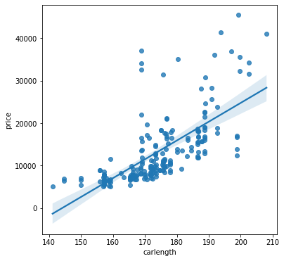
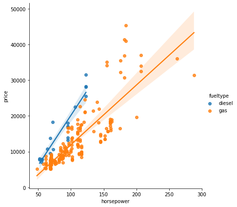
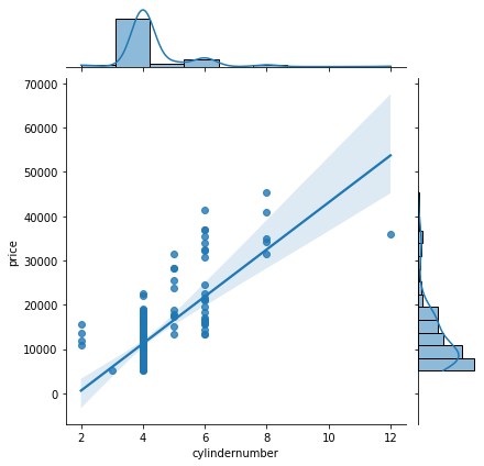
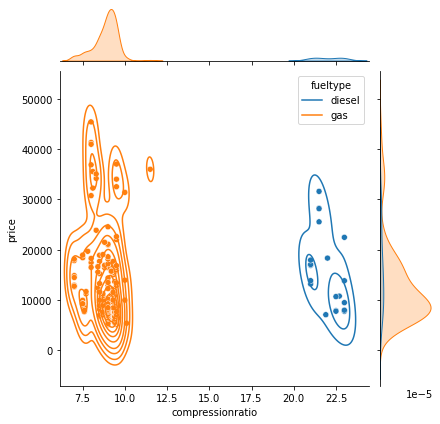
# Carlength has moderate relationship to price
plt.figure(figsize=(6,6));
sns.regplot(data=dataset, x="carlength", y="price");

# Carwidth has moderate relationship to price
plt.figure(figsize=(6,6));
sns.regplot(data=dataset, x="carwidth", y="price");

# Carweight has moderate/strong relationship to price
plt.figure(figsize=(6,6));
sns.regplot(data=dataset, x="curbweight", y="price");

# Engine size has strong relationship to price
sns.lmplot(data=dataset, x="enginesize", y="price", hue='fueltype', height=6)

# Horsepower has strong relationship to price for both fuel types
sns.lmplot(data=dataset, x="horsepower", y="price", hue='fueltype', height=6)

# Cylinder number has moderate/strong relationship to price
sns.jointplot(data=dataset, x="cylindernumber", y="price", kind="reg");

# Clear classification relationship between compressionratio and fueltype
g = sns.jointplot(data=dataset, x="compressionratio", y="price", hue='fueltype');
g.plot_joint(sns.kdeplot, hue='fueltype');

(a) Car Length vs Price

(b) Car Width vs Price

(c) Curb Weight vs Price

(d) Engine Size vs Price

(e) Horsepower vs Price

(f) Cylinder Number vs Price

(g) Compression Ratio vs Price

Figure 4. Plots for visualizing

3 Linear Regression

3.1 Univariate Models

Multiple univariate models were trained for comparison using a custom Linear Regression training function. Models were trained with ‘carlength’, ‘carwidth’, ‘curbweight’, ‘cylindernumber’, ‘enginesize’ and ‘horsepower’ independent variables. In most cases the model accuracy was the best with a 70% training and 30% testing split ( See Items 3.1.1 - 3.1.4 ). However, with engine size and horsepower models more accuracy was achieved with an 80% training and 20% testing split ( See Items 3.1.5 - 3.1.6 ).

Code

# Import regression training libraries and packages
from sklearn.model_selection import train_test_split
from sklearn.linear_model import LinearRegression
from sklearn import metrics


# Linear Regression training function that takes in X and Y arguments and displays results
def myLinRegModel(x, y, testSize):
    
    # While loop to iterate every 10% from given test size
    while testSize>0:
        
        # Splitting data into training and testing variables using the values passed into function
        x_train, x_test, y_train, y_test = train_test_split(x, y, test_size=(testSize/100), random_state=0)

        # Training model with LinearRegression function and training data
        regressor = LinearRegression()
        regressor.fit(x_train, y_train)
    
        # Print test size of current iteration
        print('Test Size:', testSize, '%\n')

        # Print intercept and CoEfficient values of model
        print("a =", regressor.intercept_)
        print("b =", regressor.coef_)

        # Test the trained model with test data and store in variable
        y_pred = regressor.predict(x_test)

        # Display predicted values next to actual values for comparison
        df = pd.DataFrame({'Actual': y_test, 'Predicted': y_pred})
        print(df)
    
        # Display accuracy of model predictions in the form of Mean Absolute Error, Mean Squared Error,
        # Root Mean Squared Error using the difference between actual and predicted values
        print('Mean Absolute Error:', metrics.mean_absolute_error(y_test, y_pred))
        print('Mean Squared Error:', metrics.mean_squared_error(y_test, y_pred))
        print('Root Mean Squared Error:', np.sqrt(metrics.mean_squared_error(y_test, y_pred)))
        print('R2 Score: ', metrics.r2_score(y_test,y_pred)*100, '%\n', sep='')
        
        # Decrease test size by 10
        testSize -= 10

3.1.1 Car Length vs Price

Code

# Carlength Column
carLength = dataset.iloc[:, 10:-15].values

# Price Column
price = dataset.iloc[:, 25].values.round(2)

# Call custom regression model function with 30% test size
myLinRegModel(carLength, price, 30)

Test Size: 30 %

a = -63541.11342037626
b = [440.33603117]
     Actual     Predicted
0    6795.0   6516.349139
1   15750.0  19153.993234
..      ...           ...
60   6479.0    131.476687
61  15510.0  18625.589997

[62 rows x 2 columns]
Mean Absolute Error: 3981.584437549869
Mean Squared Error: 32715085.38508641
Root Mean Squared Error: 5719.71025359558
R2 Score: 50.45973947401606%

Test Size: 20 %

a = -63738.09854118214
b = [441.42013341]
     Actual     Predicted
0    6795.0   6491.844685
1   15750.0  19160.602514
..      ...           ...
39  45400.0  24192.792035
40   8916.5   5079.300258

[41 rows x 2 columns]
Mean Absolute Error: 4528.295484564718
Mean Squared Error: 43469954.12056989
Root Mean Squared Error: 6593.174813439266
R2 Score: 43.84913586892223%

Test Size: 10 %

a = -66742.8631493445
b = [459.19742348]
     Actual     Predicted
0    6795.0   6315.446927
1   15750.0  19494.412981
..      ...           ...
19   6488.0   6131.767957
20   9959.0  12698.291113

[21 rows x 2 columns]
Mean Absolute Error: 3945.9317457788898
Mean Squared Error: 29396652.85426334
Root Mean Squared Error: 5421.868022578873
R2 Score: 26.410928631260454%

3.1.2 Car Width vs Price

Code

# Carwidth Column
carWidth = dataset.iloc[:, 11:-14].values

# Price Column
price = dataset.iloc[:, 25].values.round(2)

# Call custom regression model function with 30% test size
myLinRegModel(carWidth, price, 30)

Test Size: 30 %

a = -172630.60948546475
b = [2822.14912394]
     Actual     Predicted
0    6795.0   8551.364271
1   15750.0  15042.307256
..      ...           ...
60   6479.0   7704.719534
61  15510.0  15042.307256

[62 rows x 2 columns]
Mean Absolute Error: 3036.57768015824
Mean Squared Error: 22710512.087679498
Root Mean Squared Error: 4765.554751304354
R2 Score: 65.60960571372881%

Test Size: 20 %

a = -172526.22359994025
b = [2819.03318321]
     Actual     Predicted
0    6795.0   8455.706762
1   15750.0  14939.483084
..      ...           ...
39  45400.0  30444.165591
40   8916.5   6764.286852

[41 rows x 2 columns]
Mean Absolute Error: 3674.9155902799166
Mean Squared Error: 31370813.470780104
Root Mean Squared Error: 5600.965405247573
R2 Score: 59.47779746918066%

Test Size: 10 %

a = -181627.87173597398
b = [2957.89666431]
     Actual     Predicted
0    6795.0   8269.094113
1   15750.0  15072.256441
..      ...           ...
19   6488.0   6494.356114
20   9959.0  11818.570110

[21 rows x 2 columns]
Mean Absolute Error: 3197.214272696799
Mean Squared Error: 19783555.22362383
Root Mean Squared Error: 4447.87086409035
R2 Score: 50.47553663690271%

3.1.3 Curb Weight vs Price

Code

# Curbweight Column
carWeight = dataset.iloc[:, 13:-12].values

# Price Column
price = dataset.iloc[:, 25].values.round(2)

# Call custom regression model function with 30% test size
myLinRegModel(carWeight, price, 30)

Test Size: 30 %

a = -18679.037713196016
b = [12.40359272]
     Actual     Predicted
0    6795.0   4949.806413
1   15750.0  20404.682939
..      ...           ...
60   6479.0   2568.316611
61  15510.0  15530.071001

[62 rows x 2 columns]
Mean Absolute Error: 2670.404540077829
Mean Squared Error: 18443910.151758883
Root Mean Squared Error: 4294.637371392244
R2 Score: 72.0704958192619%

Test Size: 20 %

a = -18833.605447325583
b = [12.47623193]
     Actual     Predicted
0    6795.0   4933.616372
1   15750.0  20479.001353
..      ...           ...
39  45400.0  27515.596159
40   8916.5   4546.853183

[41 rows x 2 columns]
Mean Absolute Error: 3256.3206631106873
Mean Squared Error: 25249391.034916148
Root Mean Squared Error: 5024.877215904499
R2 Score: 67.3849408384091%

Test Size: 10 %

a = -19880.405624111718
b = [12.9537027]
     Actual     Predicted
0    6795.0   4796.398026
1   15750.0  20936.711595
..      ...           ...
19   6488.0   6221.305324
20   9959.0  10819.869783

[21 rows x 2 columns]
Mean Absolute Error: 2695.197926817389
Mean Squared Error: 11737364.677960433
Root Mean Squared Error: 3425.9837533123873
R2 Score: 70.61768320191304%

3.1.4 Cylinder Number vs Price

Code

# Cylinder Number Column
cylinderNumber = dataset.iloc[:, 15:-10].values

# Price Column
price = dataset.iloc[:, 25].values.round(2)

# Call custom regression model function with 30% test size
myLinRegModel(cylinderNumber, price, 30)

Test Size: 30 %

a = -8750.74345729567
b = [5045.13677503]
     Actual     Predicted
0    6795.0  11429.803643
1   15750.0  21520.077193
..      ...           ...
60   6479.0  11429.803643
61  15510.0  11429.803643

[62 rows x 2 columns]
Mean Absolute Error: 3944.3868255082953
Mean Squared Error: 26684225.038138304
Root Mean Squared Error: 5165.677597192676
R2 Score: 59.59223566856468%

Test Size: 20 %

a = -9046.162097201766
b = [5112.35112126]
     Actual     Predicted
0    6795.0  11403.242388
1   15750.0  21627.944630
..      ...           ...
39  45400.0  31852.646873
40   8916.5  11403.242388

[41 rows x 2 columns]
Mean Absolute Error: 4280.5628888250285
Mean Squared Error: 32605207.611888204
Root Mean Squared Error: 5710.096987958103
R2 Score: 57.88330998687709%

Test Size: 10 %

a = -10564.254121382277
b = [5479.84028365]
     Actual     Predicted
0    6795.0  11355.107013
1   15750.0  22314.787580
..      ...           ...
19   6488.0  11355.107013
20   9959.0  11355.107013

[21 rows x 2 columns]
Mean Absolute Error: 3464.088015146232
Mean Squared Error: 18346836.560473613
Root Mean Squared Error: 4283.32073985519
R2 Score: 54.072095495610604%

3.1.5 Engine Size vs Price

Code

# Engine Size Column
engineSize = dataset['enginesize'].values.reshape(-1, 1)

# Price Column
price = dataset.iloc[:, 25].values.round(2)

# Call custom regression model function with 30% test size
myLinRegModel(engineSize, price, 30)

Test Size: 30 %

a = -7574.131488222356
b = [163.29075344]
     Actual     Predicted
0    6795.0   7285.327074
1   15750.0  18715.679815
..      ...           ...
60   6479.0   7448.617828
61  15510.0  12184.049678

[62 rows x 2 columns]
Mean Absolute Error: 2898.9726929694702
Mean Squared Error: 14541824.65222288
Root Mean Squared Error: 3813.374444271488
R2 Score: 77.97940083865093%

Test Size: 20 %

a = -7613.370926304753
b = [164.31545176]
     Actual     Predicted
0    6795.0   7339.335184
1   15750.0  18841.416808
..      ...           ...
39  45400.0  42338.526410
40   8916.5   7175.019732

[41 rows x 2 columns]
Mean Absolute Error: 3195.031241401546
Mean Squared Error: 16835544.028987687
Root Mean Squared Error: 4103.113942969131
R2 Score: 78.25324722629195%

Test Size: 10 %

a = -8207.420855494747
b = [169.490971]
     Actual     Predicted
0    6795.0   7216.257505
1   15750.0  19080.625475
..      ...           ...
19   6488.0   7385.748476
20   9959.0  10436.585954

[21 rows x 2 columns]
Mean Absolute Error: 2877.111549011615
Mean Squared Error: 12997474.409783443
Root Mean Squared Error: 3605.2010221045157
R2 Score: 67.46323206602058%

3.1.6 Horsepower vs Price

Code

# Horsepower Column
horsepower = dataset.iloc[:, 21:-4].values

# Price Column
price = dataset.iloc[:, 25].values.round(2)

# Call custom regression model function with 30% test size
myLinRegModel(horsepower, price, 30)

Test Size: 30 %

a = -4438.686268723588
b = [170.53827527]
     Actual     Predicted
0    6795.0   7157.916450
1   15750.0  22165.284674
..      ...           ...
60   6479.0   5452.533697
61  15510.0  14320.524011

[62 rows x 2 columns]
Mean Absolute Error: 3518.2488303322393
Mean Squared Error: 25821021.51495541
Root Mean Squared Error: 5081.438921698795
R2 Score: 60.89937966412712%

Test Size: 20 %

a = -4053.153036276188
b = [166.64923709]
     Actual     Predicted
0    6795.0   7278.995086
1   15750.0  21944.127950
..      ...           ...
39  45400.0  26610.306588
40   8916.5   7612.293560

[41 rows x 2 columns]
Mean Absolute Error: 3733.6933754512147
Mean Squared Error: 29626244.692692798
Root Mean Squared Error: 5442.999604325983
R2 Score: 61.73128603174041%

Test Size: 10 %

a = -4796.241165629246
b = [174.95075436]
     Actual     Predicted
0    6795.0   7100.410131
1   15750.0  22496.076514
..      ...           ...
19   6488.0   6050.705605
20   9959.0  15498.046340

[21 rows x 2 columns]
Mean Absolute Error: 3839.1982159225827
Mean Squared Error: 26172943.363739382
Root Mean Squared Error: 5115.949898478227
R2 Score: 34.48088778430891%

3.2 Multivariate Models

Multiple univariate models were trained for comparison using a custom Linear Regression training function. Accuracy varies in each model with changes in training/test splits and would most likely would be benefitted with more rows of data ( See Items 3.2.1 - 3.2.3 ). The highest accurracy is seen with the model that takes in the most columns for the independent variables ( See Items 3.2.3 ).

3.2.1 Carlength, Carwidth, Curbweight vs Price

Code

# Create copy of dataset and drop all columns not used for multivariate regression models
datasetCopy = dataset
datasetCopy.drop(['carheight', 'enginetype', 'fuelsystem', 'boreratio', 'stroke', 'compressionratio'],\
inplace=True, axis=1)

# Store carlength, carwidth & curbweight columns in X
X1 = datasetCopy.iloc[:, 10:-7].values

# Call Regression Model Function with multiple x values & 30% test size
myLinRegModel(X1, price, 30)

Test Size: 30 %

a = -36739.21951780665
b = [-208.48890057  764.98885537   13.97180015]
     Actual     Predicted
0    6795.0   5818.760203
1   15750.0  19003.466111
..      ...           ...
60   6479.0   5929.766976
61  15510.0  13762.735333

[62 rows x 2 columns]
Mean Absolute Error: 2458.5442776902337
Mean Squared Error: 16492573.815910544
Root Mean Squared Error: 4061.1049993703123
R2 Score: 75.02539290462342%

Test Size: 20 %

a = -44634.67127094674
b = [-188.42001434  856.204069     13.34802623]
     Actual     Predicted
0    6795.0   5783.995638
1   15750.0  18977.251262
..      ...           ...
39  45400.0  29066.672270
40   8916.5   5459.428429

[41 rows x 2 columns]
Mean Absolute Error: 2943.0381053387778
Mean Squared Error: 22423198.502769
Root Mean Squared Error: 4735.313981434494
R2 Score: 71.03558082852051%

Test Size: 10 %

a = -51021.53652492876
b = [-194.19115484  961.28023332   13.59661598]
     Actual     Predicted
0    6795.0   5698.395155
1   15750.0  19277.437054
..      ...           ...
19   6488.0   6694.931234
20   9959.0  10475.100811

[21 rows x 2 columns]
Mean Absolute Error: 2357.566870487648
Mean Squared Error: 9101964.422986511
Root Mean Squared Error: 3016.9462081691995
R2 Score: 77.21491923452972%

3.2.2 Cylinder Number, Engine Size, Horsepower vs Price

Code

# Store cylindernumber, enginesize & horsepower columns in X
X2 = datasetCopy.iloc[:, 13:-4].values

# Call Regression Model Function with multiple x values & 30% test size
myLinRegModel(X2, price, 30)

Test Size: 30 %

a = -6717.131795698624
b = [-875.82889691  133.38667558   65.31455209]
     Actual     Predicted
0    6795.0   6359.129636
1   15750.0  19692.219717
..      ...           ...
60   6479.0   5839.370791
61  15510.0  13103.941091

[62 rows x 2 columns]
Mean Absolute Error: 2681.2430726638395
Mean Squared Error: 13246002.119140355
Root Mean Squared Error: 3639.505752041114
R2 Score: 79.941657245098%

Test Size: 20 %

a = -7307.824968281864
b = [-522.31275964  128.16628088   63.17240963]
     Actual     Predicted
0    6795.0   6561.779408
1   15750.0  20047.965597
..      ...           ...
39  45400.0  39099.945713
40   8916.5   6559.957946

[41 rows x 2 columns]
Mean Absolute Error: 3028.44528450474
Mean Squared Error: 15255724.671464592
Root Mean Squared Error: 3905.8577382522003
R2 Score: 80.29392621688581%

Test Size: 10 %

a = -7824.384102535303
b = [-613.42877141  135.45474355   63.82356299]
     Actual     Predicted
0    6795.0   6388.284759
1   15750.0  20259.732808
..      ...           ...
19   6488.0   6140.798124
20   9959.0  12025.455910

[21 rows x 2 columns]
Mean Absolute Error: 2944.3040595022885
Mean Squared Error: 12712894.325743863
Root Mean Squared Error: 3565.5145948016907
R2 Score: 68.17562555579416%

3.2.3 Carlength, Carwidth, Curbweight, Cylinder Number, Engine Size, Horsepower vs Price

Code

# Store carlength, carwidth, curbweight, cylindernumber,
# enginesize & horsepower columns in X
X3 = datasetCopy.iloc[:, 10:-4].values

# Call Regression Model Function with multiple x values & 30% test size
myLinRegModel(X3, price, 30)

Test Size: 30 %

a = -50133.27454870472
b = [-62.20404054 772.47835707   3.18527494  18.99449375  65.77507898
  64.33402142]
     Actual     Predicted
0    6795.0   6067.345502
1   15750.0  20331.280734
..      ...           ...
60   6479.0   5548.422659
61  15510.0  13525.755400

[62 rows x 2 columns]
Mean Absolute Error: 2536.7293535638096
Mean Squared Error: 12555624.008739235
Root Mean Squared Error: 3543.39159686581
R2 Score: 80.98709273909488%

Test Size: 20 %

a = -54793.72590677004
b = [-38.92156396 789.71920542   2.95208156 366.09875078  59.3369646
  58.3182745 ]
     Actual     Predicted
0    6795.0   6167.243070
1   15750.0  20562.635157
..      ...           ...
39  45400.0  36977.654082
40   8916.5   5783.745608

[41 rows x 2 columns]
Mean Absolute Error: 2873.7239149228203
Mean Squared Error: 16025434.859390952
Root Mean Squared Error: 4003.178094887979
R2 Score: 79.29967874050975%

Test Size: 10 %

a = -55531.82635570387
b = [-30.01857827 784.53201154   2.29960226 213.59515415  74.83936968
  58.2469381 ]
     Actual     Predicted
0    6795.0   6065.470340
1   15750.0  20665.341927
..      ...           ...
19   6488.0   5585.072554
20   9959.0  11876.766620

[21 rows x 2 columns]
Mean Absolute Error: 3020.6881171033187
Mean Squared Error: 13605511.765351668
Root Mean Squared Error: 3688.5650008304947
R2 Score: 65.94112325398689%

4 KNeigbors vs Decision Tree Classification

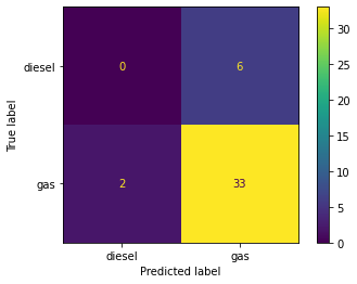
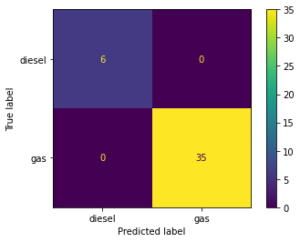
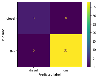
KNeigbors and Decision Tree models are trained side-by-side for comparison using a custom Classification Model training function. Items 4.1 – 4.3 display model accurracy in conjuction with data scaling strategies. Accuracy in both models improves to 100% when normalizing or standardizing data (See Figures 5, 6 & 7).

Code

# Import classification training libraries and packages
from sklearn.preprocessing import StandardScaler, MinMaxScaler 
from sklearn.neighbors import KNeighborsClassifier
from sklearn.tree import DecisionTreeClassifier
# Packages for displaying classification accuracy
from sklearn.metrics import classification_report, confusion_matrix, ConfusionMatrixDisplay
np.set_printoptions(suppress=True)

# Classification training function that takes in X values to classify according to Y values
# and takes what scalar should be used
def myClassModel(X, y, scale):
    
    # Split dataset into random train and test subsets:
    X_train, X_test, y_train, y_test = train_test_split(X, y, test_size=0.20) 

    # Standardizes data if specified when calling function
    if scale == 'Standardize':
    
        # Standardize features by removing mean and scaling to unit variance:
        scaler = StandardScaler()
        scaler.fit(X_train)
        X_train = scaler.transform(X_train)
        X_test = scaler.transform(X_test)
    
    # Normalizes data if specified when calling function
    elif scale == "Normalize":
    
        # Normalize features by shrinking data range between 0 & 1:
        scaler = MinMaxScaler()
        scaler.fit(X_train)

        X_train = scaler.transform(X_train)
        X_test = scaler.transform(X_test)

    # Use the KNN classifier to fit data:
    knclassifier = KNeighborsClassifier(n_neighbors=5)
    knclassifier.fit(X_train, y_train) 

    # Predict y data with KNN classifier: 
    y_predict = knclassifier.predict(X_test)

    # Print KNN classifier results:
    print("KNeigbors Classifier - Scaling:", scale)
    cm = confusion_matrix(y_test, y_predict, labels=knclassifier.classes_)
    disp = ConfusionMatrixDisplay(confusion_matrix=cm, display_labels=knclassifier.classes_)
    disp.plot()
    plt.show()
    print(classification_report(y_test, y_predict))
    
     # Use the Decision Tree classifier to fit data:
    dtclassifier = DecisionTreeClassifier()
    dtclassifier.fit(X_train, y_train) 

    # Predict y data with Decision Tree classifier: 
    y_predict = dtclassifier.predict(X_test)

    # Print Decision Tree classifier results:
    print("Decision Tree Classifier - Scaling:", scale)
    cm = confusion_matrix(y_test, y_predict, labels=dtclassifier.classes_)
    disp = ConfusionMatrixDisplay(confusion_matrix=cm, display_labels=dtclassifier.classes_)
    disp.plot()
    plt.show()
    print(classification_report(y_test, y_predict))

4.1 No Scaling

Code

# Store all numeric values in X
X = dataset[['wheelbase', 'carlength', 'carwidth', 'carheight',\
             'curbweight', 'cylindernumber', 'enginesize', 'boreratio',\
             'stroke', 'compressionratio', 'horsepower', 'peakrpm',\
             'citympg', 'highwaympg', 'price']].values

# Classify according to fuel type
y = dataset['fueltype']

# Call Classification Model Function with no scalar
myClassModel(X, y, 'None')

KNeigbors Classifier - Scaling: None
              precision    recall  f1-score   support

      diesel       0.00      0.00      0.00         6
         gas       0.85      0.94      0.89        35

    accuracy                           0.80        41
   macro avg       0.42      0.47      0.45        41
weighted avg       0.72      0.80      0.76        41

Decision Tree Classifier - Scaling: None
              precision    recall  f1-score   support

      diesel       1.00      1.00      1.00         6
         gas       1.00      1.00      1.00        35

    accuracy                           1.00        41
   macro avg       1.00      1.00      1.00        41
weighted avg       1.00      1.00      1.00        41

(a) KNeigbors Classifier

(b) Decision Tree Classifier

Figure 5. Classifier Models Confusion Matrices - No Scaling

4.2 Standardized Scaling

Code

# Store all numeric values in X
X = dataset[['wheelbase', 'carlength', 'carwidth', 'carheight',\
             'curbweight', 'cylindernumber', 'enginesize', 'boreratio',\
             'stroke', 'compressionratio', 'horsepower', 'peakrpm',\
             'citympg', 'highwaympg', 'price']].values

# Classify according to fuel type
y = dataset['fueltype']

# Call Classification Model Function with no scalar
myClassModel(X, y, 'Standardize')

KNeigbors Classifier - Scaling: Standardize
              precision    recall  f1-score   support

      diesel       1.00      1.00      1.00         3
         gas       1.00      1.00      1.00        38

    accuracy                           1.00        41
   macro avg       1.00      1.00      1.00        41
weighted avg       1.00      1.00      1.00        41

Decision Tree Classifier - Scaling: Standardize
              precision    recall  f1-score   support

      diesel       1.00      1.00      1.00         3
         gas       1.00      1.00      1.00        38

    accuracy                           1.00        41
   macro avg       1.00      1.00      1.00        41
weighted avg       1.00      1.00      1.00        41

(a) KNeigbors Classifier

(b) Decision Tree Classifier

Figure 6. Classifier Models Confusion Matrices - Standard Scaling

4.3 Normalized Scaling

Code

# Store all numeric values in X
X = dataset[['wheelbase', 'carlength', 'carwidth', 'carheight',\
             'curbweight', 'cylindernumber', 'enginesize', 'boreratio',\
             'stroke', 'compressionratio', 'horsepower', 'peakrpm',\
             'citympg', 'highwaympg', 'price']].values

# Classify according to fuel type
y = dataset['fueltype']

# Call Classification Model Function with no scalar
myClassModel(X, y, 'Normalize')

KNeigbors Classifier - Scaling: Normalize
              precision    recall  f1-score   support

      diesel       1.00      1.00      1.00         3
         gas       1.00      1.00      1.00        38

    accuracy                           1.00        41
   macro avg       1.00      1.00      1.00        41
weighted avg       1.00      1.00      1.00        41

Decision Tree Classifier - Scaling: Normalize
              precision    recall  f1-score   support

      diesel       1.00      1.00      1.00         3
         gas       1.00      1.00      1.00        38

    accuracy                           1.00        41
   macro avg       1.00      1.00      1.00        41
weighted avg       1.00      1.00      1.00        41

(a) KNeigbors Classifier

(b) Decision Tree Classifier

Figure 7. Classifier Models Confusion Matrices - Normalized Scaling

5 Clustering

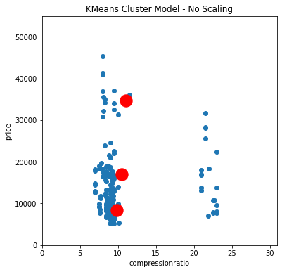
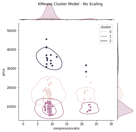
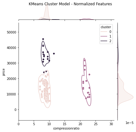
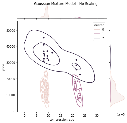
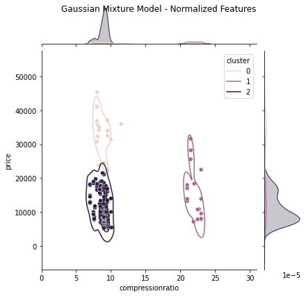
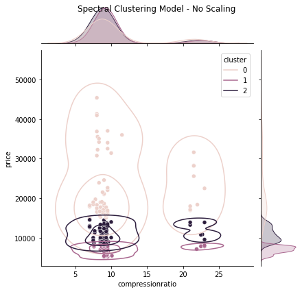
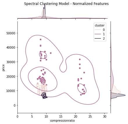
Kmeans, Gaussian Mixture and Spectral clustering models are trained using a custom cluster model training function. Items 5.1 – 5.3 display each model’s code and results when trained with unchanged data and normalized data. In all three (3) models, the “price” data heavily biased the results, which is corrected by normalizing the data providing more accuracy in each case. The spectral clustering model trained with normalized data performed marginally better than its counterparts ( See Items 5.1 – 5.3 ).

Code

# Import clustering packages
from sklearn.cluster import KMeans
from sklearn.mixture import GaussianMixture
from sklearn.cluster import SpectralClustering

# Cluster training function that takes in X values to cluster, along with
# what model should be used and how many clusters should be created
def myClusterModel(X, model, num_clusters):
    
    # Store columns names of features
    column_name = list(X.columns)
    # Stores feature values fro use in some models
    features = X.values
    
    # Takes given features and creates dataframe for some models
    X = pd.DataFrame(X)
    
    # Normalize features
    scaler = MinMaxScaler()
    scaler.fit(features)
    scaled = scaler.transform(features)
    
    # For KMeans model
    if model=='KM':
        # Initialize KMeans model with given number of clusters
        kmeans = KMeans(n_clusters=num_clusters)
        
        # Produce clusters with model and append cluster label info to DataFrame X
        X['cluster'] = kmeans.fit_predict(features)
        
        # Set plot size
        plt.figure(figsize=(6, 6))
        # Plot data with given features
        plt.scatter(X[column_name[0]], X[column_name[1]])

        # Plot KMeans cluster centers
        plt.scatter(kmeans.cluster_centers_[:, 0], kmeans.cluster_centers_[:, 1], s=300, c='red')
        # Display plot
        plt.xlabel(column_name[0])
        plt.ylabel(column_name[1])
        plt.xlim(0,31)
        plt.ylim(0,55000)
        plt.title('KMeans Cluster Model - No Scaling')
        plt.show()

        # Display scatter plot with KDE to see compare how well
        # model performed at creating relevant clusters
        g = sns.jointplot(data=X, x=column_name[0], y=column_name[1], hue='cluster')
        g.fig.suptitle("KMeans Cluster Model - No Scaling")
        g.plot_joint(sns.kdeplot, levels=3)
            
        # Delete cluster column so we can add scaled cluster labels to plot 
        X.drop('cluster', inplace=True, axis=1)
        
        # Appends new scaled cluster label info to DataFrame X
        X['cluster'] = kmeans.fit_predict(scaled)
            
        # Display scatter plot with KDE to see compare how well
        # model performed at creating relevant clusters with scaled data
        g = sns.jointplot(data=X, x=column_name[0], y=column_name[1], hue='cluster', xlim=(0,31))
        g.fig.suptitle("KMeans Cluster Model - Normalized Features")
        g.plot_joint(sns.kdeplot, levels=num_clusters)
            
    # For Gaussian Mixture model    
    elif model=='GMM':
        # Initialize Gaussian Mixture with given number of clusters
        gmm_model = GaussianMixture(n_components=num_clusters)
        gmm_model.fit(features)

        # Produce clusters with model and append cluster label info to DataFrame X
        X['cluster'] = gmm_model.predict(features)

        # Display scatter plot with KDE to see compare how well
        # model performed at creating relevant clusters
        g = sns.jointplot(data=X, x='compressionratio', y='price', hue="cluster")
        g.fig.suptitle("Gaussian Mixture Model - No Scaling")
        g.plot_joint(sns.kdeplot, levels=num_clusters, common_norm=False)
        
        # Feed scaled data into model
        gmm_model.fit(scaled)
 
        # Delete cluster column so we can add scaled cluster labels to plot
        X.drop('cluster', inplace=True, axis=1)
    
        # Appends new scaled cluster label info to DataFrame X
        X['cluster'] = gmm_model.predict(scaled)

        # Display scatter plot with KDE to see compare how well
        # model performed at creating relevant clusters with scaled data
        g = sns.jointplot(data=X, x='compressionratio', y='price', hue='cluster', xlim=(0,31))
        g.fig.suptitle("Gaussian Mixture Model - Normalized Features")
        g.plot_joint(sns.kdeplot, levels=num_clusters)
    
    elif model=='SC':
        # Initialize KMeans model with given number of clusters
        sc = SpectralClustering(n_clusters=num_clusters, random_state=25, n_neighbors=25,\
        affinity='nearest_neighbors')
        
        # Appends cluster label info to DataFrame X
        X['cluster'] = sc.fit_predict(X[[column_name[0], column_name[1]]])
        
        # Display scatter plot with KDE to see compare how well
        # model performed at creating relevant clusters
        g = sns.jointplot(data=X, x='compressionratio', y='price', hue="cluster")
        g.fig.suptitle("Spectral Clustering Model - No Scaling")
        g.plot_joint(sns.kdeplot, levels=num_clusters, common_norm=False)
        
        # Delete cluster column so we can add scaled cluster labels to plot
        X.drop('cluster', inplace=True, axis=1)
        
        # convert scaled values to dataframe to be used by model
        scaled = pd.DataFrame(scaled)
        
        # Appends new scaled cluster label info to DataFrame X
        X['cluster'] = sc.fit_predict(scaled[[0, 1]])
        
        # Display scatter plot with KDE to see compare how well
        # model performed at creating relevant clusters with scaled data
        g = sns.jointplot(data=X, x='compressionratio', y='price', hue="cluster", xlim=(0,31))
        g.fig.suptitle("Spectral Clustering Model - Normalized Features")
        g.plot_joint(sns.kdeplot, levels=num_clusters, common_norm=False)

5.1 KMeans Model

Code

# Store all features in X
X = dataset[['compressionratio', 'price']]

# KMeans Cluster Model to be used
model = 'KM'

# Number of clusters to be created
n_clusters = 3

# Call Clustering Model Function and pass in features
# model & number of clusters
myClusterModel(X, model, n_clusters)

(a) Scatter Plot - No Scaling

(b) Joint Plot - No Scaling

(c) Joint Plot - Normalized Scaling

Figure 8. KMeans Cluster Model Visualizations

5.2 Gaussian Mixture Model

Code

# Store all features in X
X = dataset[['compressionratio', 'price']]

# Gaussian Mixture Model to be used
model = 'GMM'

# Number of clusters to be created
n_clusters = 3

# Call Clustering Model Function and pass in features
# model & number of clusters
myClusterModel(X, model, n_clusters)

(a) Joint Plot - No Scaling

(b) Joint Plot - Normalized Scaling

Figure 9. Gaussian Mixture Cluster Model Visualizations

5.3 Spectral Clustering Model

Code

# Store all features in X
X = dataset[['compressionratio', 'price']]

# Spectral Clustering Model to be used
model = 'SC'

# Number of clusters to be created
n_clusters = 3

# Call Clustering Model Function and pass in features
# model & number of clusters
myClusterModel(X, model, n_clusters)

(a) Joint Plot - No Scaling

(b) Joint Plot - Normalized Scaling

Figure 10. Spectral Clustering Model Visualizations

Appendix

References

Dataset
https://www.kaggle.com/datasets/hellbuoy/car-price-prediction?select=CarPrice_Assignment.csv

Data Cleaning
https://datatofish.com/category/python/

Data Scaling
https://dataakkadian.medium.com/standardization-vs-normalization-da7a3a308c64
https://medium.datadriveninvestor.com/data-pre-processing-with-scikit-learn-9896c561ef2f

Measuring Accuracy
https://www.bmc.com/blogs/mean-squared-error-r2-and-variance-in-regression-analysis/

Visualizations
https://scikit-learn.org/stable/modules/generated/sklearn.metrics.ConfusionMatrixDisplay.html
https://seaborn.pydata.org/api.html
https://matplotlib.org/stable/api/pyplot_summary.html

Classification & Clustering Models
https://www.activestate.com/resources/quick-reads/how-to-classify-data-in-python/
https://builtin.com/data-science/data-clustering-python
https://towardsdatascience.com/machine-learning-algorithms-part-9-k-means-example-in-python-f2ad05ed5203

General Python
https://stackoverflow.com