Play Demo

Select one of the example photos or upload your own photo to test how the model classifies the image.

For more information on model deployments see Deployment section of Appendix.

Video Walkthrough

1 Project Overview

1.1 Purpose of Document

The purpose of this document is to detail the building of deep learning models using a convolutional neural network architecture. The different techniques, models and methods used to improve performance will be discussed.

2 Dataset

2.1 Bee vs Wasp

For this project I chose a Bee vs Wasp dataset found on Kaggle. I imported the dataset and created a new folder called “images” to which I added subfolders: “bee1”, “bee2”, “wasp1”, “wasp2”, “other_insect” and “other_noinsect”. The data loader in my custom train_models function then creates classes based on the folder structure and feeds that to the model. The data set itself isn’t the cleanest as it seems that some images have not been placed in the correct folder which will sometimes give the model wrong information. No doubt this will affect the accuracy that can be attained with this dataset.

Dataset

View Bee vs Wasp dataset on Kaggle.

3 Experimenting

3.1 Trial and Error

I created a custom function named train_models that I could use to conduct my tests a little faster. With a trial and error approach, I began manually trying different learning rates, model types and image sizes, along with training models with unfrozen weights ( See Figure 1, Table 1, Figure 2 & Table 2 ). Eventually I thought I should start trying to automate some of these tuning methods and, by doing so, hopefully optimize the outcomes.

Note

View full details of the trial and error testing in the Experimenting section on the Google Colab Notebook.

#Function to train models more easily
def train_models(image_size, batch_size, images_path, test_size, model_type):
    #instructions for preparing data batches, size of images
    #and normalize data
    batch_tfms = [*aug_transforms(size=image_size),Normalize.from_stats(*imagenet_stats)]

    #function for creating batches with specified parameters
    data = ImageDataLoaders.from_folder(images_path,
                                        valid_pct=test_size,
                                        ds_tfms=batch_tfms,
                                        item_tfms=Resize(460),
                                        bs=batch_size)
    
    # test whether batch function is working with parameters
    data.show_batch(max_n=9, figsize=(20,10))

    #return the trained model
    return vision_learner(data, model_type, metrics=error_rate).to_fp16()

Source: Google Colab Notebook

Code

#image size
image_size = 224

#batch size, number of images to transfer to GPU to train at one time
batch_size = 64

#Image path
images_path = "kaggle_bee_vs_wasp/images"

#test size
test_size = 0.2

#CNN model
model_type = resnet34

#Create model with dataset and parameters
learn_resnet34 = train_models(image_size, batch_size, images_path, test_size, model_type)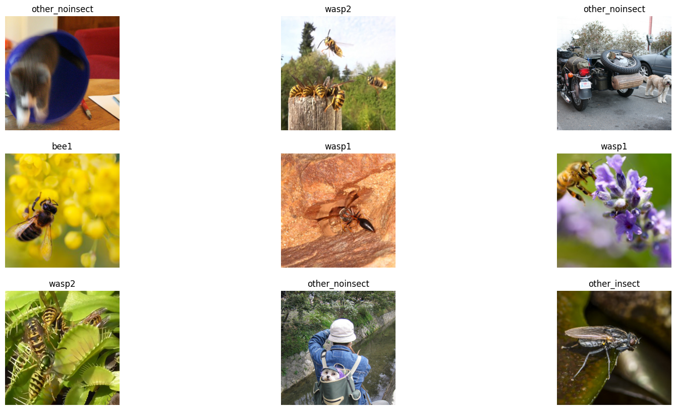

Source: Google Colab Notebook

Code

#train with discovered learning
#rates and train two more epochs... may improve accuracy
learn_resnet34.fit_one_cycle(2, lr_max=slice(1e-6,1e-3))

**Table** 1. First resnet34 best training results
epoch	train_loss	valid_loss	error_rate	time
0	0.179072	0.169389	0.055166	02:12
1	0.105617	0.161333	0.046848	02:08

Source: Google Colab Notebook

Code

#image size
image_size = 224

#batch size, number of images to transfer to GPU to train at one time
batch_size = 64

#Image path
images_path = "kaggle_bee_vs_wasp/images"

#test size
test_size = 0.2

#CNN model
model_type = resnet50

#Try resnet50 with same image size as first resnet34 tests
learn_resnet50 = train_models(image_size, batch_size, images_path, test_size, model_type)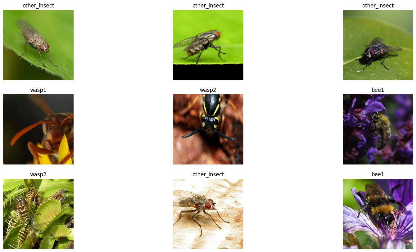

Source: Google Colab Notebook

Code

#save where the model is currently at
learn_resnet50.save('stage_2')
# freeze most of the weights again and train two more epochs
learn_resnet50.freeze()
learn_resnet50.fit_one_cycle(2)

**Table** 2. First resnet50 best training results
epoch	train_loss	valid_loss	error_rate	time
0	0.152754	0.199921	0.056918	04:58
1	0.082319	0.159553	0.042907	04:59

Source: Google Colab Notebook

3.2 Automating Hyperparameter Tuning

In research, I found a Python library called Optuna that could be used to automate hyperparameter tuning. Optuna does this by creating a “study” that runs a user specified amount of trials and uses an objective function to suggest user specified parameters to optimize for a certain metric. So in this case, I created a custom objective function named tune_hyperparameters that takes in learning rate, batch size, and weight decay parameters and returns the error rate of the model trained with those parameters. The Optuna optimize function then suggests hyperparameters that should start lowering the error rate of successive trials. I then wrote another custom function called optimization_study that ran the Optuna study using the tune_hyperparameters function. The optimization_study function also selects the trial that did the best and proceeds to unfreeze all of the weights and train the model again with the best found hyperparameters. Some of my initial tests with this automated hyperparameter tuning proved promising as I was able to get the error rate lower than I had previously gotten it.

Note

View full details of the automation testing in the Automate Hyperparameter Tuning section on the Google Colab Notebook.

# Custom function to choose the best trial and unfreeze weights to train further
def optimization_study(selected_model):

    # Create an Optuna study and optimize the objective function
    study = optuna.create_study(direction="minimize") # Minimize the error rate
    study.optimize(lambda trial: tune_hyperparameters(trial, image_size, images_path, test_size, selected_model), n_trials=3)

    # Print the best hyperparameters and the corresponding accuracy
    best_params = study.best_params
    best_error_rate = study.best_value
    print("Best Hyperparameters:", best_params)
    print("Best Accuracy:", best_error_rate)

    #retrieve best model's state dict file
    best_state_dict_file = f"{selected_model}_state_dict_trial_{study.best_trial.number}.pth"

    # Get the best trial from the study
    best_trial = study.trials[study.best_trial.number]

    # Retrieve the hyperparameters of the best trial
    hyperparameters = best_trial.params

    # Access individual hyperparameters
    learning_rate = hyperparameters["learning_rate"]
    batch_size = hyperparameters["batch_size"]
    weight_decay = hyperparameters["weight_decay"]

    #Create model with the same architecture as the best trial and load dict file into it
    best_trial_learn = train_models(image_size, batch_size, images_path, test_size, selected_model)
    best_trial_learn.model.load_state_dict(torch.load(best_state_dict_file))

    #unfreeze all weights to train with optimal hyperparameters
    best_trial_learn.unfreeze()
    # Fit the model with the best trial's hyperparameters
    best_trial_learn.fine_tune(4, base_lr=learning_rate, wd=weight_decay)

    #close it back up
    best_trial_learn.freeze()

    #return the model with all of the best results
    return best_trial_learn

Source: Google Colab Notebook

3.3 Automate Testing Different Models

As I started to achieve some good results with my automations I decided to go even further. I wrote another custom function called try_models that loops through a list of different models, runs an Optuna study on it and saves the model state from the best trial from that particular study on that particular model. Once the try_models function has finished looping through the list of models it selects the model that achieved the lowest error rate, creates a learner from that model and loads the model state of the best trial from that model. It then proceeds to unfreeze all of the weights and train the model again with hyperparameters from that particular model’s best trail. After training is complete the function freezes the weights again, displays the results, and returns the model. I found some success using this new function as long as I kept the trial size relatively low as when I increased the trial size it exponentially increases compute time and quickly reaches the limits of free tier kernels.

Note

View full details of the try_models function automation testing in the Automate testing different models section on the Kaggle Notebook.

# Custom function to try different models with the other automation functions
def try_models(image_size, images_path, test_size, models, trial_size):
    best_trials = {}
    for model in models:
        best_trials[model.__name__] = optimization_study(image_size, images_path, test_size, model, trial_size)
        
    best_overall = min(best_trials,  key=lambda x: best_trials[x].value)
    lowest_model = best_trials[best_overall]
    print("\n\nBest Overall Model:", lowest_model.user_attrs['model'].__name__)
    print("Error Rate:", lowest_model.value)
    print("Load Model's state and retrain with best hyperparameters")
    
    
    #retrieve best model's state dict file
    best_state_dict_file = f"/kaggle/working/{lowest_model.user_attrs['model'].__name__}_state_dict_trial_{lowest_model.number}.pth"

    
    # Retrieve the hyperparameters of the best trial
    hyperparameters = lowest_model.params

    # Access individual hyperparameters
    learning_rate = hyperparameters["learning_rate"]
    batch_size = hyperparameters["batch_size"]
    weight_decay = hyperparameters["weight_decay"]

    #Create model with the same architecture as the best trial and load dict file into it
    best_model_learn = train_models(image_size, batch_size, images_path, test_size, lowest_model.user_attrs["model"])
    best_model_learn.model.load_state_dict(torch.load(best_state_dict_file))

    #unfreeze all weights to train with optimal hyperparameters
    best_model_learn.unfreeze()
    # Fit the model with the best trial's hyperparameters
    best_model_learn.fine_tune(1, base_lr=learning_rate, wd=weight_decay)

    #close it back up
    best_model_learn.freeze()
    
    # Evaluate the model on the validation set
    best_error_rate = best_model_learn.validate()[1]
    
    print(f"\n\nFinal result after training model "+lowest_model.user_attrs['model'].__name__+" with:")
    print("Hyperparameters:", hyperparameters)
    print("Error Rate:", best_error_rate)

    
    #return the model with all of the best results
    return best_model_learn

Source: Kaggle Notebook

3.4 Data Augmentation

I also briefly experimented with some data augmentation, namely randomly cropping to a 224x224 image size and introducing a random horizontal flip to the images. Tests with this didn’t seem to yield any improved results, in fact it seems it may have adversely affected model performance in training. I theorize that this didn’t have much effect because the dataset already possesses a great deal of randomness so injecting more isn’t advantageous.

4 Kernels

4.1 Usage Limits

Very early on it was clear that usage limits of free tier kernels would significantly limit the ability to experiment, test and iterate. For this reason, the approach was taken to use more than one kernel so that when one reached its limit the other could be used to continue with the project. Google Colab and Kaggle were both used to complete this project and in the following two items ( 4.2 Google Colab & 4.3 Kaggle ) in this section I detail what each kernel was primarily used for. A notebook from each kernel is provided in this project submission, with Part 1 and Part 3 being included in the Google Colab notebook and Part 2 being included in the Kaggle notebook.

4.2 Google Colab

I started my initial experimentation in Google Colab and that is why it starts with the heading Part 1. Part way through the refinement of my custom automation functions I reached my limit with Google Colab so Part 2 of my code is found in the Kaggle notebook. The final part of my testing and code can be found under Part 3 of the Google Colab notebook. In Part 3, I decided to purchase some Pay-As-You-Go compute so that I could continue the rest of my project without further delays.

4.3 Kaggle

The Kaggle notebook starts with the heading of Part 2 as it is the point where I switched from Google Colab. The Kaggle notebook only includes one part and it is where most of the refinements on my custom functions can be found. I was able to make some fairly large tests at the end of the Kaggle notebook but then reached my limit. At this point I switched back to finish things off in my Google Colab notebook under Part 3.

5 Performance

To improve performance SqueezeNet, EfficientNet, Resnet and VGG models were tested along with various batch sizes, learning rates and weight decays. Two (2) different image sizes were tested: (1) 224x224 and (2) 896x896. The parameters that yielded the worst ( See Item 5.1 ) and best ( See Item 5.2 ) results are detailed in the items below.

Note

View full details of testing all of the custom automated optimization functions altogether in Part 3 of the Google Colab Notebook.

5.1 Worst Performance

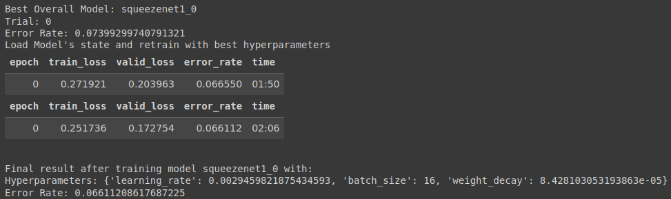
I wasn’t able to test VGG16 to long before I ran into limit restrictions on the kernel but it wasn’t performing all that well from what was seen. Further investigation would be required to confirm that VGG16 is not a good model for this dataset. SqueezeNet models did not perform as well as the other models which is not surprising giving the size and architecture of SqueezeNet models ( See Figure 3 ). The 896x896 image size did not seem to yield better results and neither did batch sizes 16 and 64. Learning rate range 1e-5 - 1e-1 did not yield good results as well as weight decay range 1e-5 – 1e-3.

**Figure** 3. Best SqueezeNet model results after optimization automations were the worst results.

5.2 Best Performance

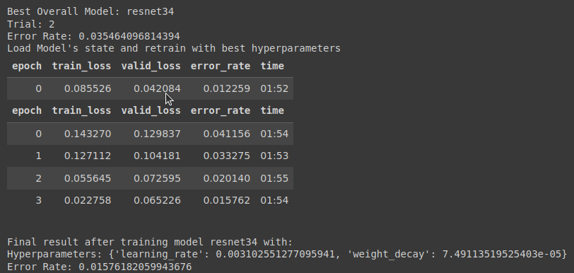
After studying some of the tests I started to isolate that a batch size of 32 did consistently well. Along with training only with a 32 batch size I narrowed the learning rate range to 1e-3 – 1e-2 and the weight decay range to 1e-5 -1e-4 as these ranges seems to provide the best results. In the end of all my testing the best performance I achieved was from a Resnet32 model trained with a 224 image size, 32 batch size, a learning rate of 3.102551277095900e-3 and a weight decay of 7.49113519525403e-05. This yielded a model with a training loss of 0.022758, valid loss of 0.065226, and error rate of 0.015762. These results show that the model is slightly overfitted but performing quite well. ( See Figure 4 )

**Figure** 4. Best Resnet model results after optimization automations were the best performance.

Appendix

Model Training Video Walkthrough

References

Optimization Library
https://optuna.org/

Deployment

Deployment Source Code

View the source code for the model deployment on HuggingFace repository.

Gradio App

View Gradio app for model deployment hosted on HuggingFace.

Deployment Resources

Hugging Face - AI community & place to host ML deployments
https://huggingface.co/

Gradio - Open-source Python library used to build machine learning/data science demos & web applications
https://www.gradio.app/